Fast Analysis of Multi-Layered Anisotropic Electromagnetic Propagation Based on Z-Transform Finite-Difference Time-Domain Method with Scale-Compressed Technique

I.   Introduction

Computational electromagnetics plays a crucial role in contemporary scientific research, especially in the design about the integrated chip when facing multi-layered problems. Due to the anisotropic complexity and directional uncertainty, many researchers and scientists are facing the computational challenge so that more mature and reliable numerical methods need to be developed to discover the propagation problems for electromagnetic fields. Those common and popular methods including finite-difference time-domain (FDTD) method [1], [2] finite-element (FEM) [3], [4] method, and integral equation (IE) methods [5], [6], have undergone decades of development to apply into a series of commercial software such as XFDTD, HFSS and FEKO. With the development of the information age, it is essential to record and process time-domain signals on computers, but these technologies are often isolated for the physical research. Fortunately, early in 1992, Sullivan [7]-[9] firstly apply Z-transform technology with FDTD, named as Z-FDTD, to achieve the union between the digital signal processing and electromagnetic simulation. The unique advantage of Z-transform in dealing with the frequency domain characteristics of dispersive media is that its introduction not only improves the numerical stability of the algorithm, but also significantly enhances computational efficiency.

After that, researchers have gradually carried out Z-FDTD method in more detailed electromagnetic applications. In 2005, Veysel et al. [10] derive the scattering field formula applicable to dispersive media by the Z-FDTD. Two years later, Yan et al. [11] propose a normalized Z-FDTD method to handle the interaction between electromagnetic waves and unmagnetized plasma. In the next year, Nadobny et al. [12] first employ the three-dimensional (3-D) FDTD with tensor formula to model inhomogeneous media and acquire the characterization from some electrical losses. In 2011, Jeng [13] independently put forward a novel closed-form expression for the 3-D dyadic FDTD-compatible Green’s function in infinite free space via a novel approach with the ordinary Z-transform along with the spatial partial difference operators. In 2015, Tomasz et al. [14] come up with time-domain discrete Green’s function using a multi-dimensional Z-FDTD with 3-D grids. In 2020, Feng et al. [15] employ the direct Z-transform technology to discretize the perfectly matched layer (PML) and truncate the FDTD region. In 2023, Zhou et al. [16] have established a 2^nd-order bilinear Z-transform method for handling the magnetized plasma based on Maxwell’s equations. However, there is still a certain gap in all those methods for solving the fully anisotropic problems. How to apply Z-FDTD to analyze electromagnetic problems with full anisotropies is currently a more reliable technological requirement.

To understand the plane waves, scientists concern the fixed wave vectors in the horizontal plane. Date back to 1994, Ren et al. [17] and Harms et al. [18] utilize Bloch-Floquet periodic boundary conditions (BPBCs) which derived from the FDTD approach in 2-D and 3-D simple isotropic cases, respectively. Four years later, Roden et al. [19] and Holter et al. [20] expand time-domain analysis in the oblique incidence to frequency domain and understand the energy transfer. Nowadays, many anisotropic materials have been discovered in nature or produced in laboratories. You et al. [21] summarized the research progress of electromagnetic metamaterials from classical to quantum fields, and researchers focus more on detecting electromagnetic propagation in anisotropy. Early in 2009, Geng et al. [22] derive the expansion coefficients of electromagnetic fields in uniaxial anisotropies or free space, which can describe the antennas’ propagation in coated impedance spheres. At the same period, Wang et al. [23] and Liang et al. [24] research multi-layered biaxial anisotropies with oblique incidence assembled by 2-D and 3-D FDTD methods, respectively. In 2020, Zhang et al. [25] implement the earliest proposal to introduce anisotropies into the periodic FDTD algorithm. Two years later, Zhan et al. [26] propose a discontinuous Galerkin time-domain method that is highly effective for some large-scale problems in the anisotropies. However, the low efficiency can be avoided as they focus on the 3-D model in those methods which occupy more computer resources. In terms of the 3-D integrated circuits, complex multi-layered problems must be more discussed in the energy transfer. In 2002, Moss et al. [27] investigate the numerical dispersion in the FDTD algorithm for layered anisotropies. To further accelerate the computational efficiency, Yang et al. [28] adopt FFT method to analyze the electromagnetic propagation embedded in a single-layer uniaxial anisotropy, while Han et al. [29] research the electromagnetic scattering with the layered uniaxial anisotropies by BCGS-FFT method. In 2021, Zhang et al. [30] firstly realize transfer matrix method under the multi-layered fully anisotropic conditions by the reliable elimination method and obtain the reliable accuracy inform the popular software COMSOL in extremely short time. In 2023, Wang et al. [31] develop spectral element spectral integration method for solving the periodic anisotropic objects about multi-layered fully anisotropies. Fatih et al. [32] proposed a 3-D subgrid algorithm for analyzing electromagnetic scattering and radiation problems, which significantly reduces computation time and memory usage while ensuring results accuracy. In 2024, N. Feng et al. [33] apply the space mapping method for solving 3-D multi-layered lossy media. Obviously, almost all those complex multi-layered anisotropic problems are executed and restricted by the frequency-domain algorithm, so that it exists still one of hard works for capturing precise data in the time domain when the electromagnetic waves go through the fully anisotropies in the short time.

For the above conventional method, it is necessary to design a 3-D model which increases the computational procedure and occupies huge computer resources to a great extent. To further simplify those difficulties, we combine a novel and reliable scale-compressed technology (SCT) with Z-FDTD method, which is named as SCT-Z-FDTD, to capture the data in time- and frequency-domain in the short time and efficiently obtain the energy transfer from complex multi-layered anisotropies illuminated by the oblique plane waves. The current algorithm exhibits strong applicability in regular and uniform hierarchical media structures, a conclusion that has been thoroughly validated in this paper. The contributions in this article are as follows:

(a) Employing Z-transform technique, four electromagnetic constitutive tensors, including relative permittivity, magnetic permeability, electrical loss and magnetic loss, are defined in the FDTD formula to excite the numerical computation.

(b) The scale-compressed technique (SCT) is proposed for converting the 3-D complex multi-layer model into the 1-D case on the condition that the plane waves can be set by the fixed transverse vectors (k_x, k_y), hence lowering the computer memory and obtain the 3-D transfer data.

(c) The SCT-Z-FDTD algorithm, which combines the SCT and Z-FDTD method, is developed to acquire additional time-domain transmission through multiple fully anisotropies under oblique incidence.

(d) It has been demonstrated that constructing a super multi-layer anisotropic model verified by the popular software COMSOL, which prove that the proposed method showcased the marked advantages of lower memory and shorter duration than the COMSOL’s work in finite frequency points.

The structure of the article is depicted as follows: In section II, we introduce the corresponding Z-transform relation about the four electromagnetic constitutive tensors under the fully anisotropic cases. In section III, given the SCT condition from the differential tensor, Z-FDTD can be constructed by the new relationships, while those formula about the electromagnetic fields (E, H) and fluxes (D, B) can be obtained in every time steps. In section IV, under the same condition of the oblique incidence, three different multi-layered models are designed and simulated by the proposed SCT-Z-FDTD methods which are compared by the software COMSOL in the reasonable error analysis. Finally, we draw the conclusions in section V.

II.   Z-Transform Relation for Fully Anisotropies

1   General Z-transform relation

One of popular techniques is the Z-transform for handling discrete signals in the time domain. By combining it with the FDTD method, the electromagnetic parameters of frequency dependent media can be converted from the frequency domain to the Z-domain so that it is crucial to comprehend how the discrete time-domain and Z-domain representations relate to one another. The Z-transform in the shifted sequence is equal to its product in the original sequence and ${{\textit{z}}^{ - m}}$ as below:

As the 2^nd numerical derivative at n^th time step can be obtained by

the relation from equation (1) and (2) can be transferred by Z-transform and satisfied as

Hence, there is equivalence among the time-domain derivative, frequency-domain operator and an algebraic expression in Z-domain as

2   Z-transform in anisotropic maxwell’s equations

In the free space or complex materials, the electromagnetic alternating conversion can be easily occurred between the electric fields E and the magnetic fields H, which can be explained by anisotropic Maxwell’s curl equations as below

where the constitutive relationship can be expressed as

which involve dielectric tensor $\boldsymbol{\varepsilon}$, magnetic permeability tensor ${\boldsymbol{\mu}}$, conductivity tensor $\boldsymbol{\sigma}_e$ and equivalent magnetic loss tensor $\boldsymbol{\sigma}_m$, respectively. Those tensors satisfy coefficient matrices of 3×3 as below

As the variables $\boldsymbol{\sigma}_e$ and $\boldsymbol{\sigma}_m$ are the frequency-dependent physical quantities, the electric flux D in frequency domain can be depicted as

where the subscript r means the relative parameter for the dielectric tensor ${\boldsymbol{\varepsilon}}$ in different materials. The auxiliary vector A_e can be obtained from the conductivity tensor ${{\boldsymbol{\sigma}} _e}$ as

Taking advantage of equation (6), the auxiliary vector A_e can be shifted from frequency domain to the Z-domain, which can be seen

After the formula simplification from equations (11) and (13), the electric fields E can be expressed as

Here, employing the Z-transform method, the equations (13) and (14) can be converted into the discrete time domain, which can be expressed as

where the 3×3 coefficient matrices R_E, Q_E can be given as

Anisotropic Maxwell’s curl equations still present the obvious duality for the electric fields E and the magnetic fields H, so that we can acquire the similar expression for the magnetic anisotropies as follow

where the corresponding 3×3 coefficient matrices R_H, Q_H can be given as

III.   Theoretical Derivation of SCT-Z-FDTD

1   Scale-compressed technology for curl operator

Left-hand side of the equations (7) and (8) are conducted by the curl operator which can described by antisymmetric tensor

Generally, in spatial region, the fields W for plane waves can be defined as

where the vector W can be represented as electric fields E or magnetic fields H, and the vector k = (k_x, k_y, $k_{\textit{z}}$)^T and r = (x, y, ${\textit{z}}$)^T are recorded as the wave and position vectors in general 3-D space. Assuming that the stationary state exists at the xOy plane with the fixed transverse wave vectors (k_x, k_y), the partial derivative in x- and y-direction can be replaced by

On the other hand, the partial derivative $\partial _{\textit{z}}$ keeps the original form to express the field’s time-domain variation along the vertical direction so that the modified matrix C is obtained as

Hence, the 3-D Maxwell’s curl equations can be successfully compressed by the substitution of transverse wave vectors (k_x, k_y) into the 1-D cases to further capture the 3-D time-domain data and understand the electromagnetic propagation in a short time, so that we employ the equation (24) to handle the antisymmetric tensor C and refer to this computational method as scale-compression technique (SCT). In our article, we adopt the Z-FDTD to implement the multi-layered model to capture 3-D propagation data, which is called as SCT-Z-FDTD method.

2   Derivation of SCT-Z-FDTD in single anisotropy

Observed by the Maxwell’s curl equations (7) and (8), it can be found that the antisymmetric tensors C are located at the left-hand side, which can act on the fields W as follow

To further construct the staggered Yee’s cells, we record the spatiotemporal nodes in Table 1 to ensure stable computation for the SCT-Z-FDTD.

Table  1.  Spatiotemporal Nodes for Yee’s Cells in the SCT-Z-FDTD

Components		Fields and Fluxes
	Time Nodes	Spatial Nodes
(E, D)	n	(Ex, Dx)	(Ey, Dy)	(Ez, Dz)
		k	k	k+1/2
(H, B)	n+1/2	(Hx, Bx)	(Hy, By)	(Hz, Bz)
		k+1/2	k+1/2	k

 | Show Table

DownLoad: CSV

In accordance with the time nodes and simplified the Maxwell’s curl equations (7) ~ (8), the electromagnetic fluxes (D, B) are obtained by the matrix form as

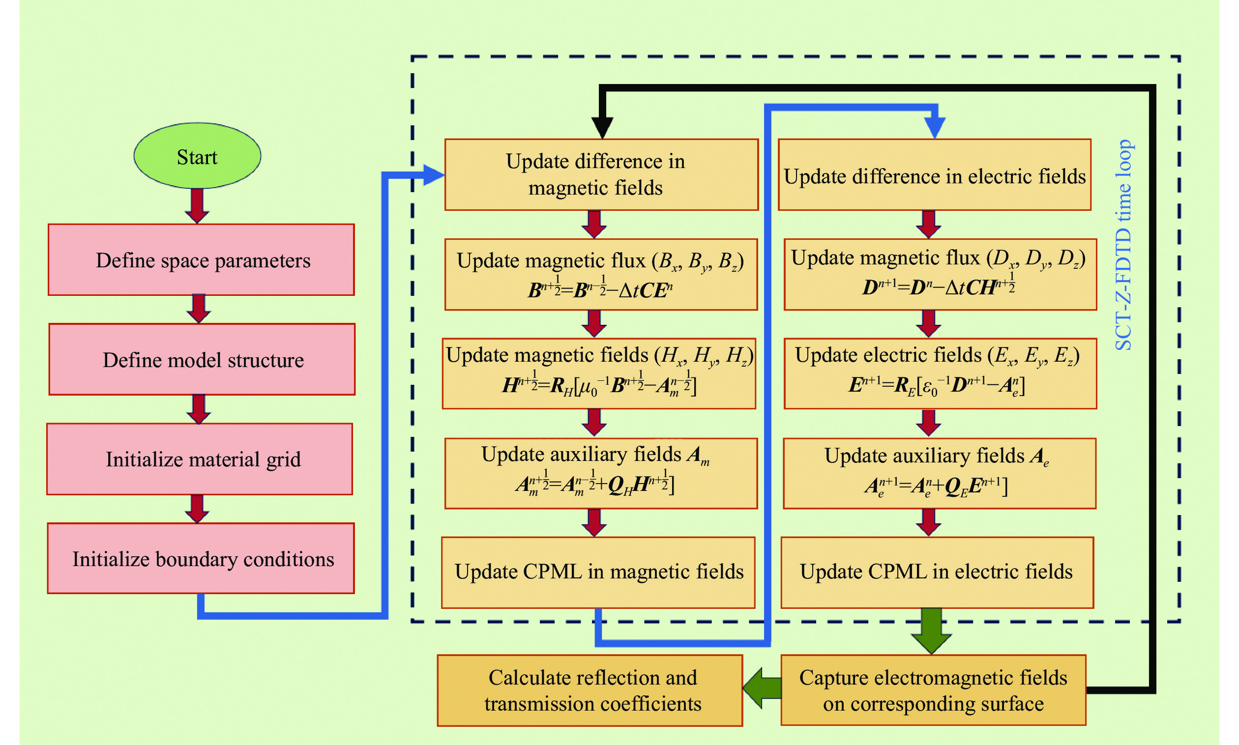
Therefore, the whole process of SCT-Z-FDTD method can be shown in Figure 1. In the first place, the geometric definition and boundary condition initialization of the model are executed before entering the SCT-Z-FDTD loop. During each cycle of the computation, the difference terms in the composition of the curl matrix are updated first. With the alternating definition of the time steps, the fields (E, H) can be underwent updating, which involve with the fluxes (D, B) and the auxiliary vectors (A_e, A_m). To vanish the reflection in the computation region, the convolutional PMLs are employed as absorption boundary which are located at top and buttom regions in the ${\textit{z}}$-direction. Given the reasonable position selection of incident, reflective and refractive surfaces, the propagation coefficients can be computed by recording the electromagnetic fields (E, H) through the multi-layered media.

Figure  1.  Flow chart of the iterative procedure for SCT-Z-FDTD method

DownLoad: Full-Size Img PowerPoint

Utilizing the spatial and temporal nodes from the Table I, update equations for electromagnetic fluxes (D, B) in each direction are expressed as

After expanding the equations (15) and (18), the conversion relationships from the fluxes (D, B) to the fields (E, H) and are employed to acquire the updated equations as

All the electromagnetic fields (E, H) are restricted for the 3×3 tensor which satisfies the anisotropic relation in each direction, so that it is necessary to execute average processing on the Yee’s cells. Therefore, the electromagnetic fields (E, H) in each direction can be represented as

At that time, the single component of auxiliary vectors (A_e, A_m) in x-direction when facing the anisotropic matrices (Q_E, Q_H) can be expressed as

Combining with the Yee’s cells, the auxiliary vectors (A_e, A_m) in x-direction can be finally recorded as

The other auxiliary vectors (A_e, A_m) in y- and ${\textit{z}}$-directions can be obtained by the similar processes from equations (58)-(65). The proposed SCT-Z-FDTD method can be executed by the above ways to capture the time-domain data and detect the propagation results based on the Fourier transform.

3   Calculation of propagation coefficients

The layered medium with the different physical variations is the main factor to emphasize the fields’ computations for assessing the propagation coefficients in the presence of anisotropies. When oblique incident waves interact with the different surface from the anisotropic medium, it will induce the reflection and refraction in the co-, cross-, and vertically polarized directions, while the shaded region in this model represents the multilayered anisotropic structures. For exciting the SCT-Z-FDTD, Gaussian pulse is employed with complex modulation expressed as

where the f₀ is modulation frequency, t presents the time step when the t₀ and τ are time constants.

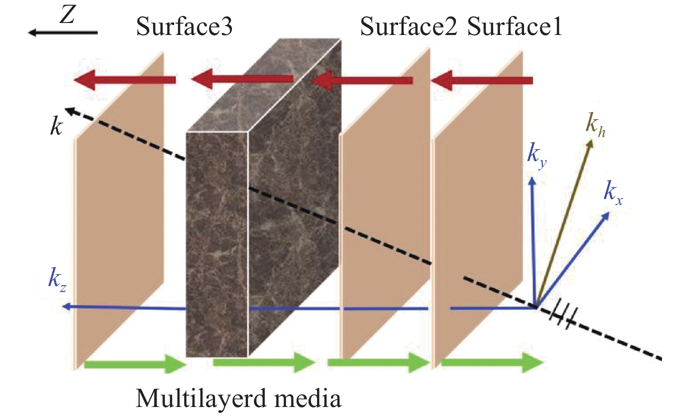
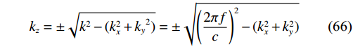
As depicted in Figure 2, to excite the fields in computational region, we choose the surface 1 as the incident location with the source defined by equation (66) shocking along the ${\textit{z}}$-axis. After the electromagnetic waves touch the multi-layer media, the total reflection waves return back to the right-hand side across the surface 2, while the total refraction waves spread towards the left region through the surface 3. In the air or vacuum, wave vector k = (k_x, k_y, ${k_{\textit{z}}}$) satisfy the dispersion relation for the oblique incidence and can be expressed as

Figure  2.  Schematic diagram for capturing the propagation coefficients through the multi-layered media.

DownLoad: Full-Size Img PowerPoint

For implementing the effective propagation, the longitudinal wave vector ${k_{\textit{z}}}$ must be a real number so that the minimum threshold for the cutoff frequency can be determined by:

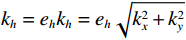
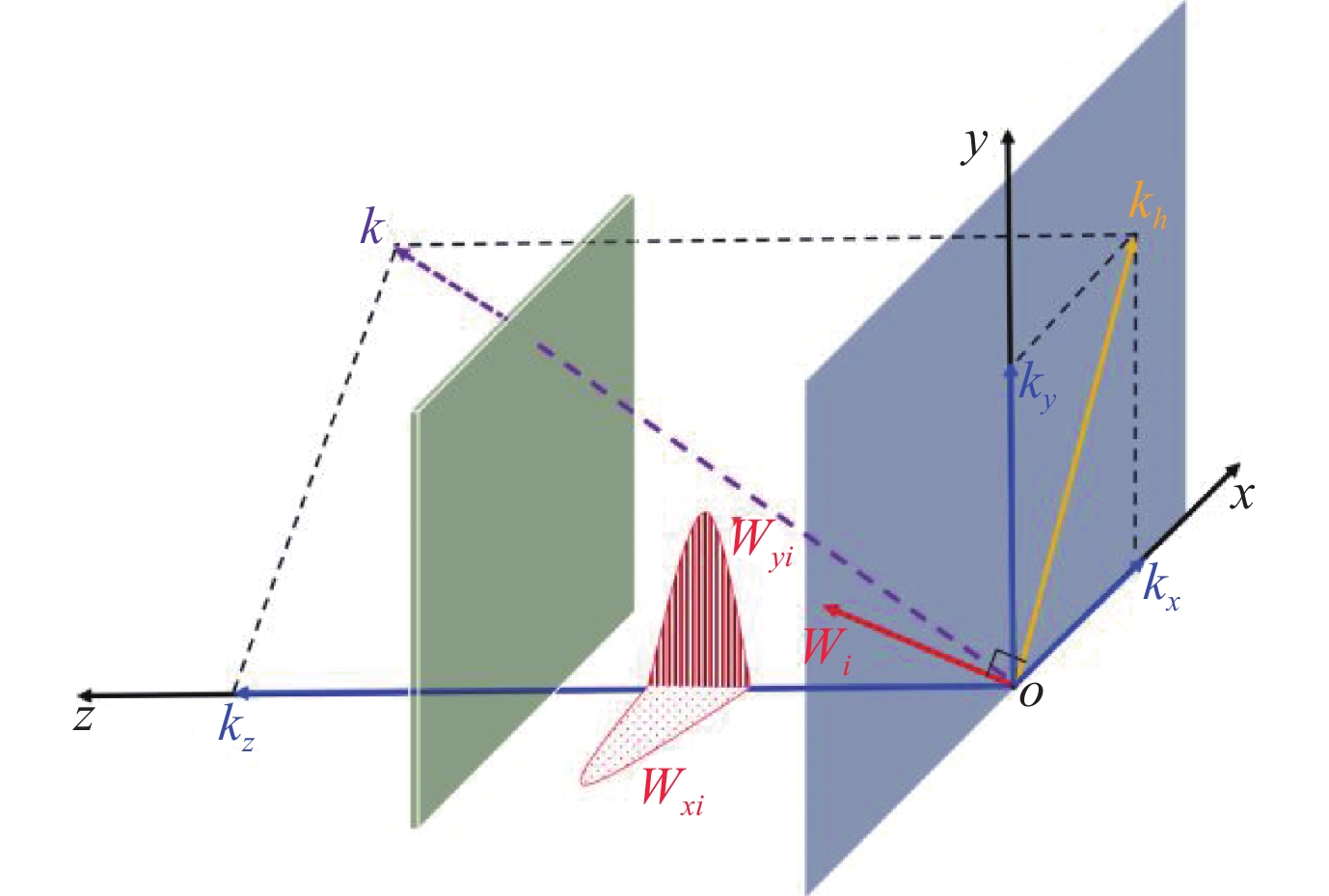
In spatial incidence, the incident electric field E_i (in TEM or TE mode) or magnetic field H_i (in TM mode) is excited on the surface 1 when executing SCT-Z-FDTD method with a fixed horizontal wave number (k_x, k_y). The plane waves enter the air with a transverse wave vector (k_x ≠ 0, k_y ≠ 0), from which the transverse angle θ = arctan (k_y/k_x) can be calculated. By computing the tangential fields of the incident waves from the surface 1, it can be seen that the non-propagating direction of the incident fields are (W_xi, W_yi) = (−W_i sinθ, W_i cosθ) as illustrated in Figure 3. Obviously, for the non-zeros variable k_z, the overall transverse wave vector ${k_h} = {e_h}{k_h} = {e_h}\sqrt {k_x^2 + k_y^2}$ are located on the xOy plane which is coplanar with (W_xi, W_yi) = (−E_xi, E_yi) in TE mode or (W_xi, W_yi) = (−H_xi, H_yi) in TM mode.

Figure  3.  Schematic diagram for oblique incidence.

DownLoad: Full-Size Img PowerPoint

To further implement the SCT-Z-FDTD method and detect the energy transfer, we choose the propagation coefficients including reflection and refraction based on three different polarizations, including the co-, cross-, and vertical direction, are recorded separately, as shown below:

where the variable W_s,p presents the amplitude for the electric fields E in TE/TEM mode or the magnetic fields H in TM mode, W_1,p denotes incident fields, specifically. The subscript p = co, cr or ve can represent the co-, cross-, and vertical polarizations while another subscript s = 2, 3 can correspond to the number of surfaces in the Figure 2. Obviously, the electric fields E, magnetic fields H and total wave vector k = (k_x, k_y, k_z) are perpendicular to each other while it occurs the vertical component E_z for TM mode or H_z for TE mode. After the SCT-Z-FDTD computation, the variables R and T represent the reflection and refraction coefficients to discover the wave’s energy transfer, respectively.

IV.   Numerical Examples

In the above sections, we have introduced the SCT-Z-FDTD method for solving electromagnetic propagation problems for the multi-layered lossy anisotropies. In this section, compared with the software COMSOL and analytical solutions, we will provide three different numerical cases to verify the effectiveness when executing our proposed method to capture the propagation coefficients. Each case, which involve three incident modes (TEM, TE and TM), demonstrate three distinct periodic media structures within the intermediate layer, as illustrated in Figure 2.

For the TEM mode with the transverse wave vector (k_x, k_y) = (0, 0), the incident fields (E, H) are parallel to the xOy plane. For the oblique incidence, TE mode with non-zero transverse wave vector (k_x, k_y) feature that co-polarized electric fields E_co and cross-polarized magnetic fields H_cr are coplanar at the xOy plane, while the vertically polarized H_ve is shocked along the z-axis. Similarly for the TM mode, the transverse wave vector keeps the status (k_x, k_y) ≠ (0, 0) while the orthogonal relation is maintained among the co-polarized magnetic fields H_co, cross-polarized electric fields E_cr and vertically electric fields E_ve. For constructing the 3D multi-layered anisotropic model, the software COMSOL with its robust modeling capabilities and precise numerical advantage is employed as the reference solution by calculating the norm error which is expressed as

All the numerical examples are executed on a workstation using AMD Ryzen 7 5800H with Radeon Graphics CPU and 512GB RAM. For ensuring computational efficiency and accuracy, our proposed SCT-Z-FDTD method is successfully implemented by computer underlying language Fortran on the compilation platform Visual Studio 2019.

1   Multi-layered periodic biaxial anisotropies

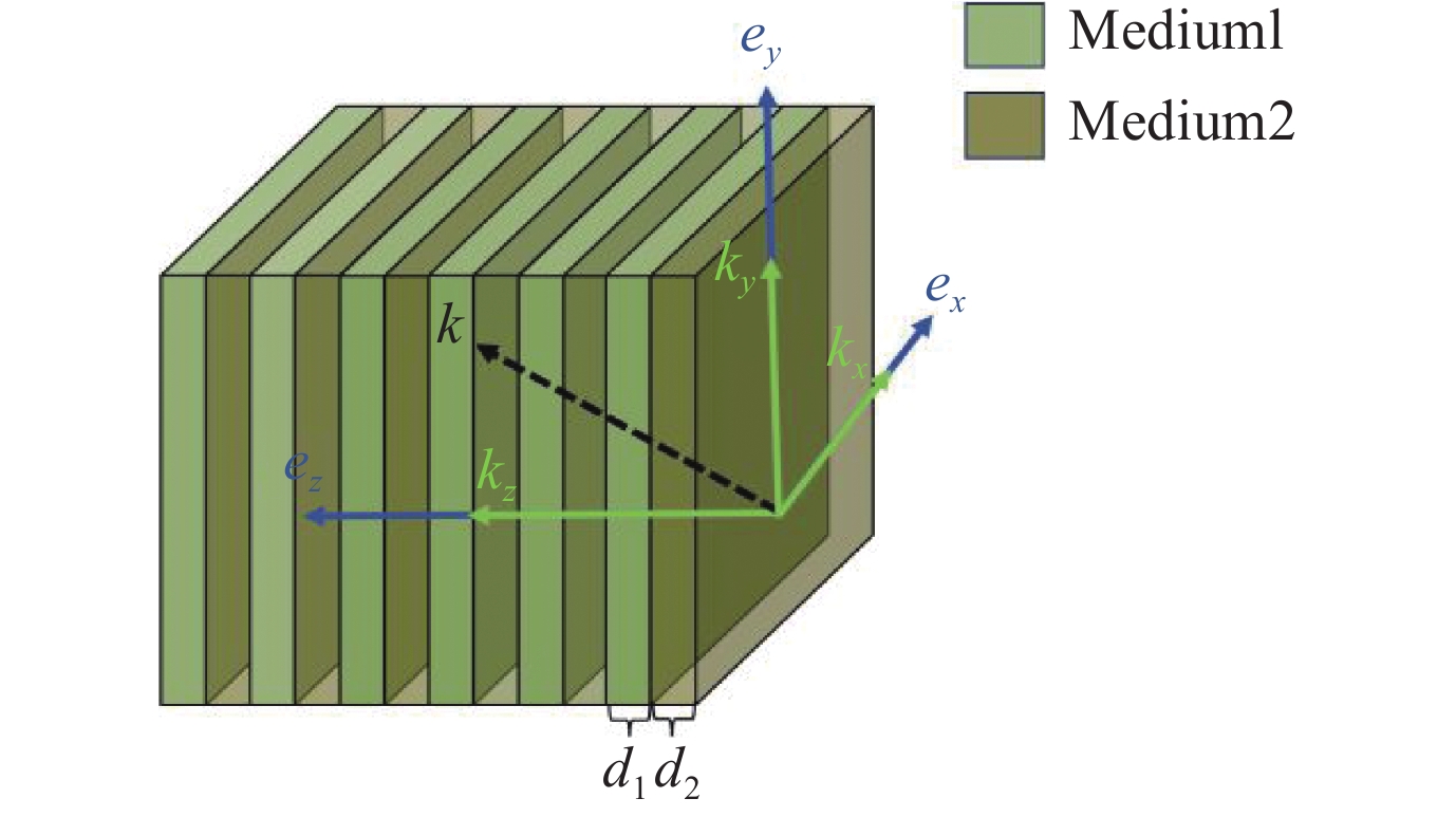
As shown in Figure 4 and Table 2, two kinds of different biaxial anisotropies are selected to design a 12-layered model with the total thickness 1.2cm, which include the thickness d₁ = d₂ = 1mm for Medium 1 and Medium 2. Three kinds of plane waves as the incidence are given in this multi-layered model to further detect the energy transfer process.

Figure  4.  Schematic diagram for periodic biaxial anisotropies

DownLoad: Full-Size Img PowerPoint

Table  2.  The medium parameters of periodic biaxial anisotropies

	ε	μ	σe	σm
Medium 1	$\left[ {\begin{array}{*{20}{c}} {7.7}&0&0 \\ 0&{3.2}&0 \\ 0&0&{1.5} \end{array}} \right]$	$\left[ {\begin{array}{*{20}{c}} {{8}{.3}}&{0}&{0} \\ {0}&{{5}{.2}}&{0} \\ {0}&{0}&{{2}{.3}} \end{array}} \right]$	$\left[ {\begin{array}{*{20}{c}} {{0}{.051}}&{0}&{0} \\ {0}&{{0}{.026}}&{0} \\ {0}&{0}&{{0}{.017}} \end{array}} \right]$	$\left[ {\begin{array}{*{20}{c}} {360}&0&0 \\ 0&{240}&0 \\ 0&0&{110} \end{array}} \right]$
Medium 2	$\left[ {\begin{array}{*{20}{c}} {5.56}&0&0 \\ 0&{3.25}&0 \\ 0&0&{2.34} \end{array}} \right]$	$\left[ {\begin{array}{*{20}{c}} {4.73}&0&0 \\ 0&{3.24}&0 \\ 0&0&{1.23} \end{array}} \right]$	$\left[ {\begin{array}{*{20}{c}} {0.031}&0&0 \\ 0&{0.018}&0 \\ 0&0&{0.022} \end{array}} \right]$	$\left[ {\begin{array}{*{20}{c}} {237}&0&0 \\ 0&{168}&0 \\ 0&0&{76} \end{array}} \right]$

 | Show Table

DownLoad: CSV

As the normal incidence, the transverse wave vector (k_x, k_y) = (0, 0), resulting in only non-zero vertical wave vector k_z, can be preset for the air background so that we can define the frequency range [0 GHz, 10 GHz] which is considered in this

TEM model. Therefore, the incident electromagnetic fields (E_i, H_i) are located at the plane xOy which we can the lateral angle θ_E = arctan2 − 90°to designate the angle between the electric fields E_i and x-axis.

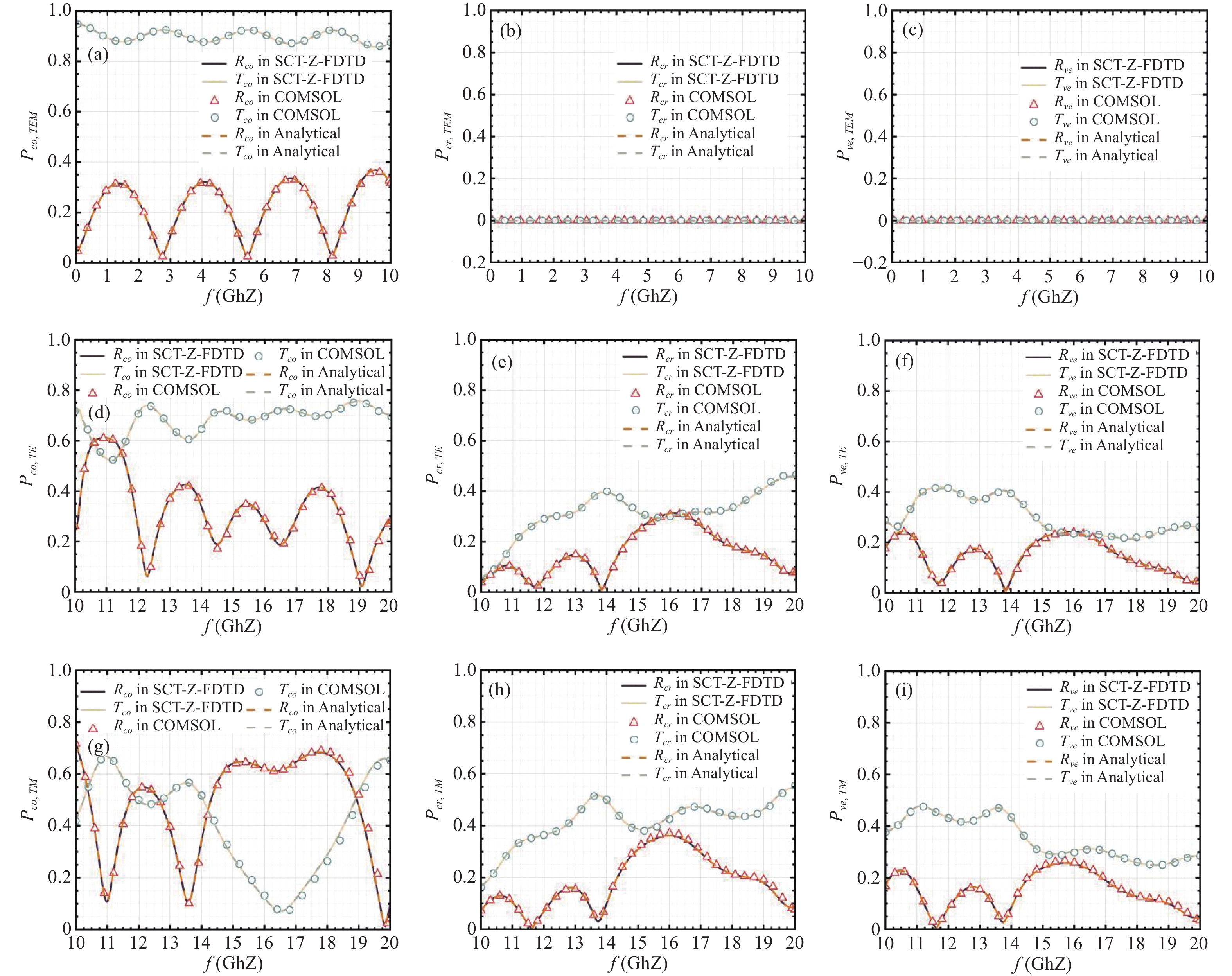
Compared with the COMSOL and analytical solutions, those numerical results are consistent with the theoretical as shown in Figure 5 (a), (b) and (c). For further capturing the propagation coefficients in oblique incidence, the transverse wave vector k_h,TE = (80, 190) or k_h,TM = (90, 170) are selected and discussed, separately in TE or TM mode. Here, we choose a new frequency range [10GHz, 20GHz] which is restricted by those minimum frequency (f_min,TE, f_min,TM) = (9.8364GHz, 9.1779GHz) based on the equation (68). After the numerical verification with software COMSOL and analytical solutions, those comparisons are depicted in Figure 5 (d), (e) and (f) for the TE mode and Figure 5 (g), (h), and (i) for the TM mode.

Figure  5.  Propagation coefficients of biaxial anisotropic periodic models: (a) R_co and T_co for TEM mode; (b) R_cr and T_cr for TEM mode; (c) R_ve and T_ve for TEM mode; (d) R_co and T_co for TE mode; (e) R_cr and T_cr for TE mode; (f) R_ve and T_ve for TE mode; (g) R_co and T_co for TM mode; (h) R_cr and T_cr for TM mode; (i) R_ve and T_ve for TM mode.

DownLoad: Full-Size Img PowerPoint

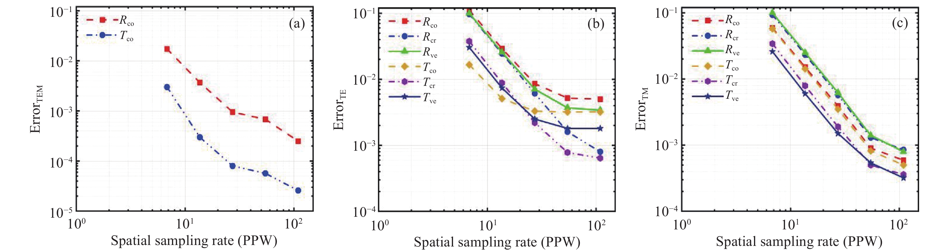
Observing the different results from the Figure 5, all those propagation coefficients maintain the sufficient numerical consistency between the proposed SCT-Z-FDTD method and the software COMSOL. For verifying the numerical accuracy of the proposed SCT-Z-FDTD method, the norm error curves are depicted from the Figure 6 with the different spatial sampling rate [6.81, 13.64, 27.27, 54.55, 109.09] PPW, which are based on its reference solution at 150 PPW and maintain the 2^nd-order convergence for the different cases. Except that the SCT-Z-FDTD method has the high precision with reasonable numerical convergence, the computational performances with the fixed spatial sampling rate have been recorded in the Table 3 which provide the ratio between the SCT-Z-FDTD and COMSOL. It can be seen that the computer memory and norm errors in SCT-Z-FDTD is significantly reduced because of the lower grid numbers and higher spatial sampling rate, while the computer time can be markedly declined due to the scale compression replacing the 3-D calculation in 1-D case. All these conclusions show the SCT-Z-FDTD’s advantages for capturing and analyzing multi-layered biaxial anisotropic model.

Figure  6.  Norm error curves of biaxial anisotropic periodic models with spatial sampling rate [6,110] PPW: (a) R_co and T_co in TEM mode; (b) R_co, T_co, R_cr, T_cr, R_ve and T_ve in TE mode; (c) R_co, T_co, R_cr, T_cr, R_ve and T_ve in TM mode.

DownLoad: Full-Size Img PowerPoint

Table  3.  The computational performance between COMSOL and SCT-Z-FDTD for the multilayered biaxial anisotropies.

Mode	Method	CPU Numbers	Spatial Sampling Rate	Grid Numbers	Computer Memory	CPU Time	Norm Error (R)
TEM	COMSOL	8	5 PPW	34548	2.18 GB	244s	1.2×10−3
	SCT-Z-FDTD	1	27.27 PPW	994	212 MB	1.406s	9.5×10−4
	Ratio		545%	2.86%	9.49%	0.58%
TE	COMSOL	8	5 PPW	102308	4.25 GB	815s	5.66×10−3
	SCT-Z-FDTD	1	27.27 PPW	994	238 MB	1.374s	7.26×10−3
	Ratio		545%	0.97%	5.47%	0.17%
TM	COMSOL	8	5 PPW	103326	3.78 GB	883s	3.85×10−2
	SCT-Z-FDTD	1	27.27 PPW	994	242 MB	1.124s	5.26×10−3
	Ratio		545%	0.96%	6.25%	0.13%

 | Show Table

DownLoad: CSV

2   Sandwich Periodic Structures with Fully Anisotropies

Without loss of generality, we increase the computational complexity by adapting a new 5-layered model where its cycle basic components are biaxial anisotropies on both sides clamping with the 1-layered fully anisotropy nested in the middle as seen in Figure 7 and Table 4, which depict that the thickness of d₁ is 0.1mm, d₂ is 0.15 mm and the total thickness become 5(d₁ + d₂ + d₁) = 1.75 cm when implementing periodic arrangement.

Figure  7.  Schematic diagram for sandwich periodic structure

DownLoad: Full-Size Img PowerPoint

Table  4.  The medium parameters of periodic sandwich structure

	ε	μ	σe	σm
Medium 1	$\left[ {\begin{array}{*{20}{c}} {8.45}&0&0 \\ 0&{3.27}&0 \\ 0&0&{2.12} \end{array}} \right]$	$\left[ {\begin{array}{*{20}{c}} {6.72}&0&0 \\ 0&{4.34}&0 \\ 0&0&{1.66} \end{array}} \right]$	$\left[ {\begin{array}{*{20}{c}} {0.028}&0&0 \\ 0&{0.015}&0 \\ 0&0&{0.024} \end{array}} \right]$	$\left[ {\begin{array}{*{20}{c}} {356}&0&0 \\ 0&{216}&0 \\ 0&0&{88} \end{array}} \right]$
Medium 2	$\left[ {\begin{array}{*{20}{c}} {1.3}&{0.11 + 0.02{\mathrm{j}}}&{0.03 + 0.2{\mathrm{j}}} \\ {0.11 - 0.02{\mathrm{j}}}&{5.25}&{0.05 + 0.2{\mathrm{j}}} \\ {0.03 - 0.2{\mathrm{j}}}&{0.05 - 0.2{\mathrm{j}}}&{7.3} \end{array}} \right]$	$\left[ {\begin{array}{*{20}{c}} {2.6}&{0.21 + 0.05{\mathrm{j}}}&{0.04 + 0.12{\mathrm{j}}} \\ {0.21 - 0.05{\mathrm{j}}}&{4.5}&{0.14 + 0.25{\mathrm{j}}} \\ {0.04 - 0.12{\mathrm{j}}}&{0.14 - 0.25{\mathrm{j}}}&{6.8} \end{array}} \right]$	$\left[ {\begin{array}{*{20}{c}} {0.0046}&{0.042}&{ - 0.013} \\ { - 0.042}&{0.038}&{0.008} \\ {0.013}&{ - 0.008}&{0.0079} \end{array}} \right]$	$\left[ {\begin{array}{*{20}{c}} {280}&{58}&{ - 52} \\ { - 58}&{115}&{82} \\ {52}&{ - 82}&{20} \end{array}} \right]$
Medium 3	$\left[ {\begin{array}{*{20}{c}} {6.27}&0&0 \\ 0&{4.56}&0 \\ 0&0&{2.31} \end{array}} \right]$	$\left[ {\begin{array}{*{20}{c}} {7.75}&0&0 \\ 0&{5.16}&0 \\ 0&0&{2.31} \end{array}} \right]$	$\left[ {\begin{array}{*{20}{c}} {0.024}&0&0 \\ 0&{0.031}&0 \\ 0&0&{0.027} \end{array}} \right]$	$\left[ {\begin{array}{*{20}{c}} {378}&0&0 \\ 0&{125}&0 \\ 0&0&{114} \end{array}} \right]$

 | Show Table

DownLoad: CSV

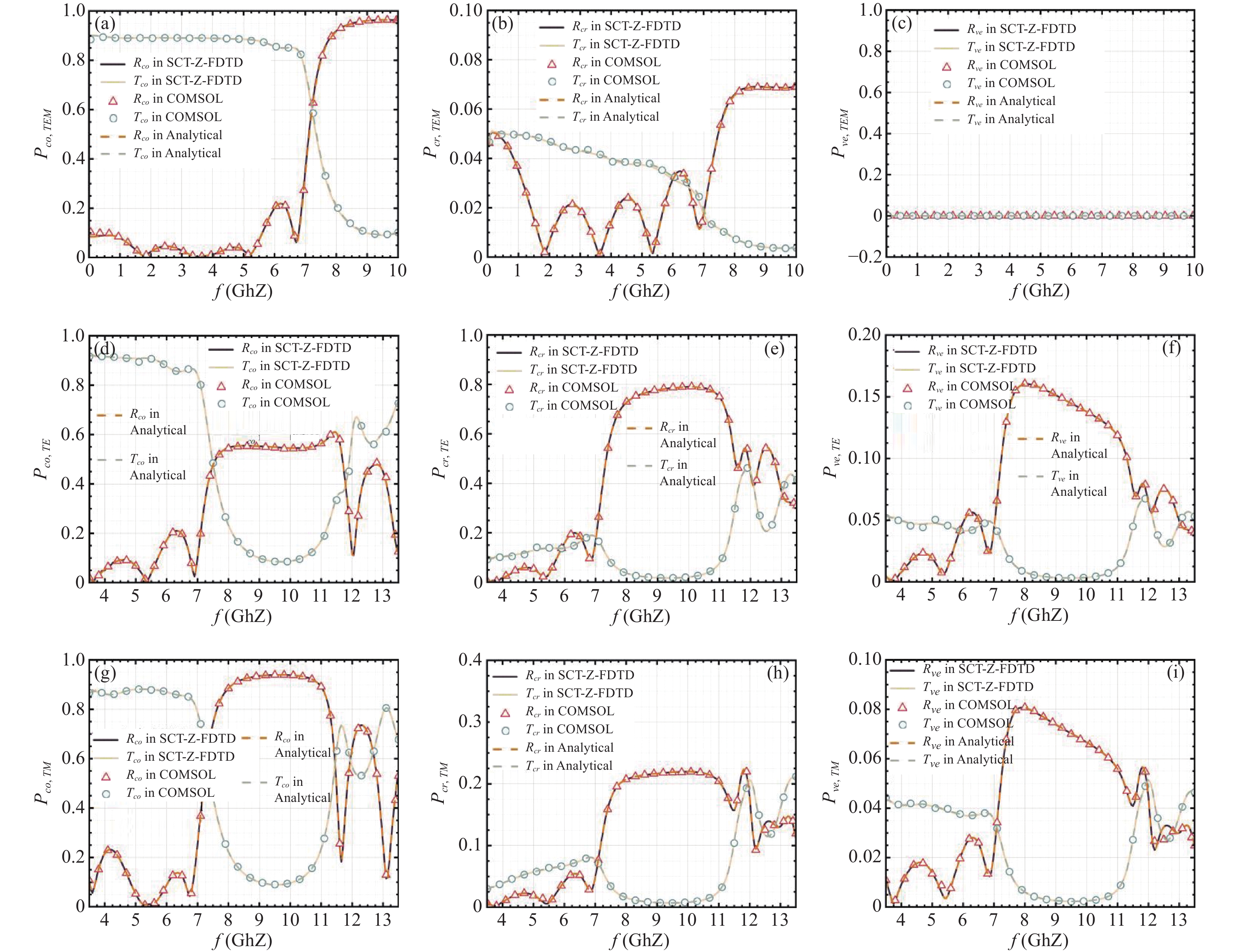
When facing the normal incidence, the transverse wave vectors (k_x, k_y) are both zero which can allow us to select a frequency range [0GHz, 10GHz] in this multi-layered model. Consequently, the incident electromagnetic fields (E_i, H_i) are confined to the xOy plane, where we designate the lateral angle θ_E = arctan2 − 90° as the angle between the electric field E_i and the x-axis. Those numerical data are in agreement with the results from the software COMSOL, as shown in Figure 8 (a), (b), and (c). To explore the propagation coefficients under oblique incidence, we separately consider transverse wave vectors k_h,TE = (20, 30) and k_h,TM = (10, 60) when discussing corresponding TE and TM mode. As constrained by minimum frequencies (f_min,TE, f_min,TM) = (1.7215GHz, 2.9043GHz), we rechoose a frequency range from 3.5GHz to 13.5GHz and present those energy transfer data which are described in Figure 8 (d), (e), and (f) for the TE mode, and Figure 8 (g), (h), and (i) for the TM mode. Examining Figure 8 across various modes, all the results reveal consistent propagation coefficients between the proposed SCT-Z-FDTD method, COMSOL and analytical solutions.

Figure  8.  Propagation coefficients of sandwich biaxial and fully anisotropic periodic models: (a) R_co and T_co for TEM mode; (b) R_cr and T_cr for TEM mode; (c) R_ve and T_ve for TEM mode; (d) R_co and T_co for TE mode; (e) R_cr and T_cr for TE mode; (f) R_ve and T_ve for TE mode; (g) R_co and T_co for TM mode; (h) R_cr and T_cr for TM mode; (i) R_ve and T_ve for TM mode.

DownLoad: Full-Size Img PowerPoint

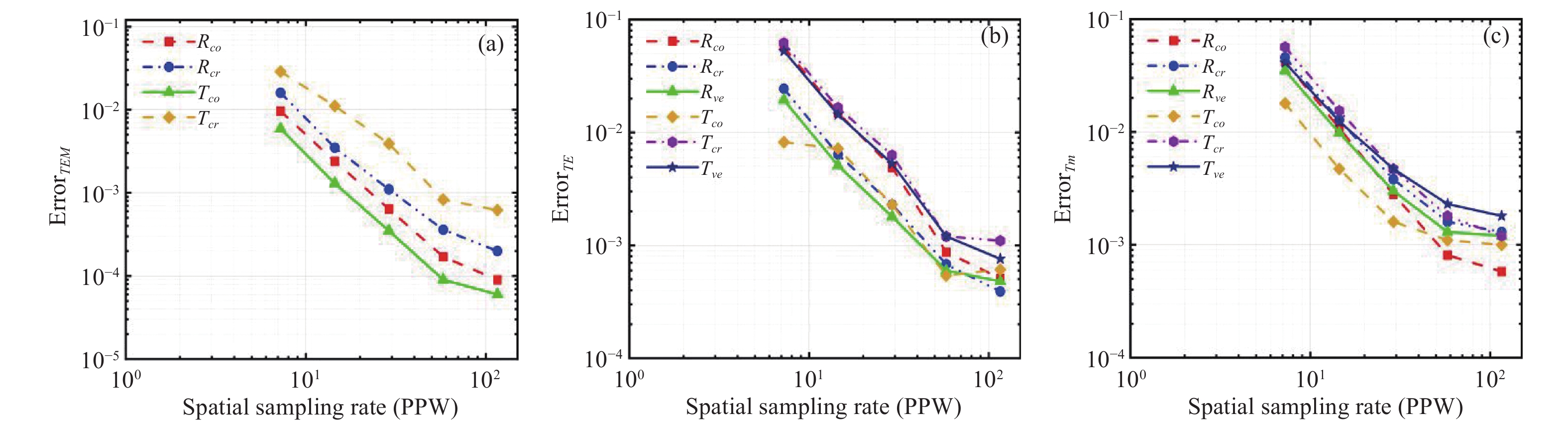
To verify the numerical accuracy about SCT-Z-FDTD, we decide the spatial sampling rates [7.23, 14.47, 28.93, 57.87, 115.75] PPW to observe the different curves of norm errors which are compared with a more-precise solution with SCT-Z-FDTD at 145 PPW, demonstrating 2^nd convergence across different incident modes as shown in Figure 9. In addition to its high precision, the SCT-Z-FDTD method offers outstanding computational efficiencies in the Table V which indicates that SCT-Z-FDTD still work for an extremely short time under single-core operation even though the commercial software COMSOL offers the multi-core parallel computation. Notably, SCT-Z-FDTD achieves significant reductions in computer memory utilization without complex grid optimization, while computational time is notably decreased by transitioning from 3-D calculations to a more efficient 1-D approach.

Figure  9.  Norm error curves of sandwich periodic models with spatial sampling rate [6,120] PPW: (a) R_co, T_co, R_cr and T_cr in TEM mode; (b) R_co, T_co, R_cr, T_cr, R_ve and T_ve in TE mode; (c) R_co, T_co, R_cr, T_cr, R_ve and T_ve in TM mode.

DownLoad: Full-Size Img PowerPoint

Table  5.  The computational performance between COMSOL and SCT-Z-FDTD for the multilayered sandwich anisotropies.

Mode	Method	CPU Numbers	Spatial Sampling Rate	Grid Numbers	Computer Memory	CPU Time	Norm error (R)
TEM	COMSOL	8	15 PPW	385298	5.22GB	3887s	6.45×10−3
	SCT-Z-FDTD	1	28.93 PPW	994	238MB	3.874s	1.22×10−3
	Ratio		192.86%	0.26%	4.45%	0.09%
TE	COMSOL	8	15 PPW	385260	7.31GB	3851s	5.4×10−3
	SCT-Z-FDTD	1	28.93 PPW	1170	268MB	4.282s	3×10−3
	Ratio		192.86%	0.30%	3.58%	0.11%
TM	COMSOL	8	15 PPW	385260	6.77GB	5064s	1.45×10−2
	SCT-Z-FDTD	1	28.93 PPW	1106	264MB	3.782s	3.2×10−3
	Ratio		192.86%	0.28%	3.81%	0.07%

 | Show Table

DownLoad: CSV

3   Periodic Structure with fully Anisotropies

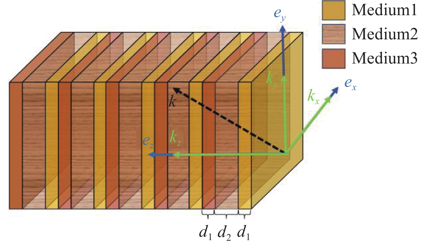
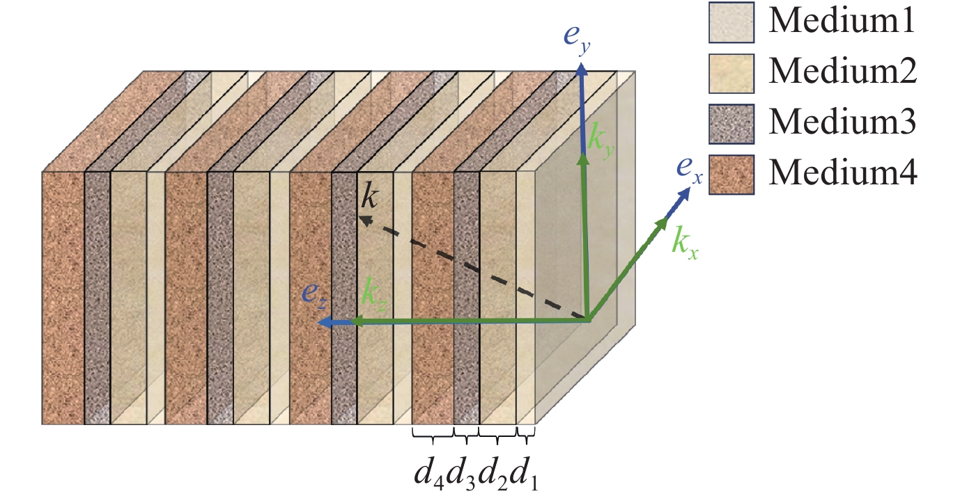
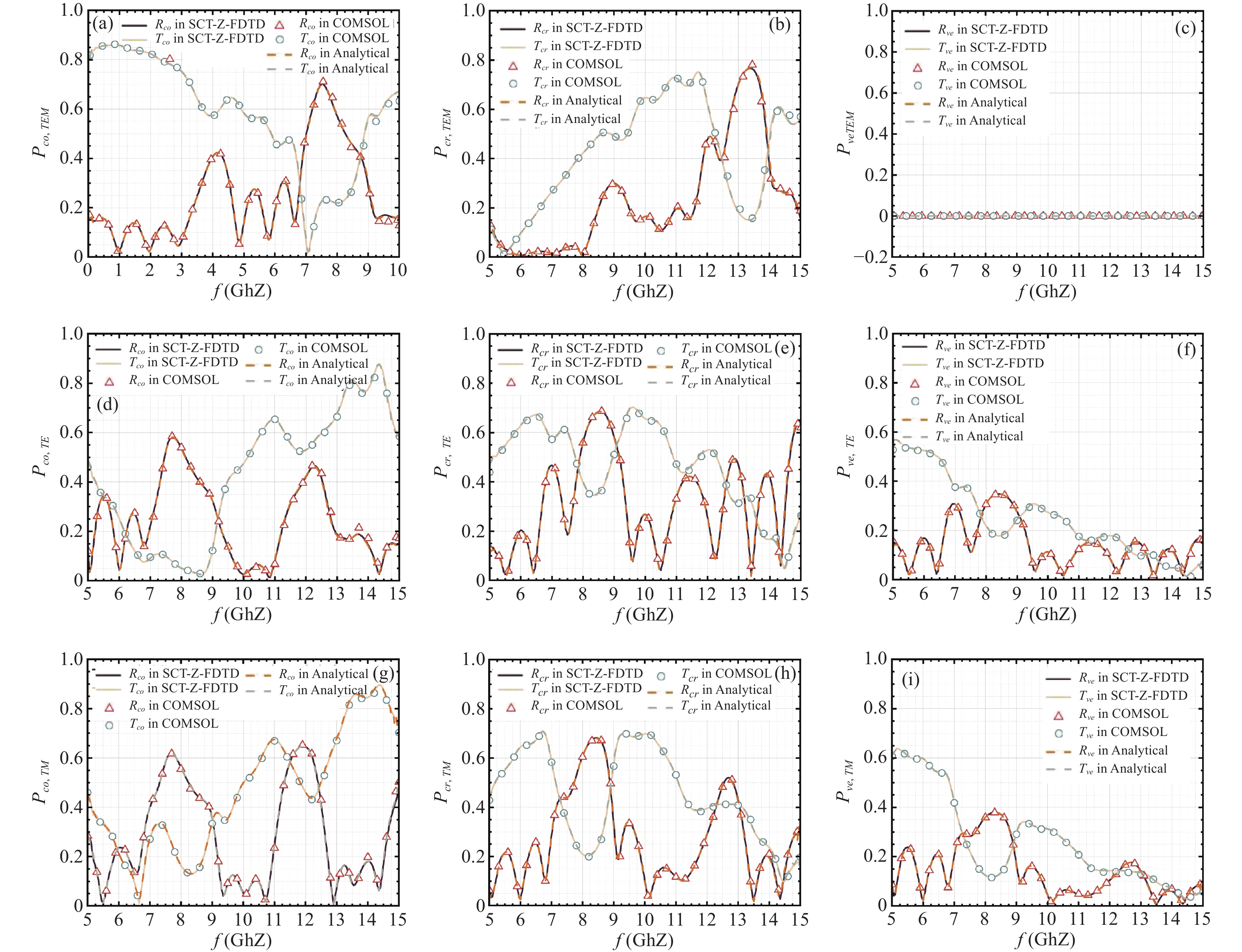
For further detecting more sophisticated media, we expand the electromagnetic discussion which is considered in more-layered fully anisotropies. As illustrated in Figure 10 and Table 6, the model involves four distinct fully tensor anisotropies to construct the most complex periodic structure, with thicknesses of d₁ = 3 mm, d₂ = 2 mm, d₃ = 2.5 mm, and d₄ = 2 mm for each layer of media, arranged periodically in 4 cycles to form a media layer with the total thickness of 3.6 cm. Here, we still delimit the frequency range [0 GHz, 10 GHz] within our TEM model with the lateral angle θ_E = arctan2 − 90° to denote the angle between the electric field E_i and the x-axis. Those results are illustrated in Figure 11 (a), (b), and (c), demonstrating consistency with results obtained from COMSOL and analytical solutions. To analyze propagation coefficients under oblique incidence, we examine k_h,TE = (40, 70) or k_h,TM = (30, 80) separately for TE and TM modes. Given a frequency range [5GHz, 15GHz] and bounded by (f_min,TE, f_min,TM) = (3.8467GHz, 4.0766GHz), it can be found that the data from the oblique incidence keep the coincidence which are depicted in Figure 11(d), (e), and (f) and Figure 11(g), (h), and (i), following the execution of the COMSOL software and calculations based on analytical solutions.

Figure  10.  Schematic diagram for multi-layer fully anisotropies

DownLoad: Full-Size Img PowerPoint

Table  6.  The medium parameters of fully periodic anisotropies

	ε	μ	σe	σm
Medium 1:	$\left[ {\begin{array}{*{20}{c}} {2.3}&{0.15 + 0.01j}&{0.02 + 0.3j} \\ {0.15 - 0.01j}&{5.65}&{0.01 + 0.02j} \\ {0.02 - 0.3j}&{0.01 - 0.02j}&{6.5} \end{array}} \right]$	$\left[ {\begin{array}{*{20}{c}} {3.6}&{0.14 + 0.2j}&{0.02 + 0.12j} \\ {0.14 - 0.2j}&{2.7}&{0.16 + 0.15j} \\ {0.02 - 0.12j}&{0.16 - 0.15j}&{6.5} \end{array}} \right]$	$\left[ {\begin{array}{*{20}{c}} {0.0054}&{0.033}&{ - 0.015} \\ { - 0.033}&{0.063}&{0.007} \\ {0.015}&{ - 0.007}&{0.0085} \end{array}} \right]$	$\left[ {\begin{array}{*{20}{c}} {340}&{78}&{ - 50} \\ { - 78}&{66}&{120} \\ {50}&{ - 120}&{290} \end{array}} \right]$
Medium 2:	$\left[ {\begin{array}{*{20}{c}} 4&{0.2 + j}&{0.1 - 0.8j} \\ {0.2 - j}&3&{0.05 + 0.2j} \\ {0.1 + 0.8j}&{0.05 - 0.2j}&2 \end{array}} \right]$	$\left[ {\begin{array}{*{20}{c}} 2&{0.05 - 0.5j}&{0.1 + 0.6j} \\ {0.05 + 0.5j}&3&{0.2 - 0.1j} \\ {0.1 - 0.6j}&{0.2 + 0.1j}&4 \end{array}} \right]$	$\left[ {\begin{array}{*{20}{c}} {0.003}&{0.05}&{ - 0.08} \\ { - 0.05}&{0.0009}&{0.02} \\ {0.08}&{ - 0.02}&{0.005} \end{array}} \right]$	$\left[ {\begin{array}{*{20}{c}} {30}&{1300}&{ - 200} \\ { - 1300}&{90}&{ - 600} \\ {200}&{600}&{100} \end{array}} \right]$
Medium 3:	$\left[ {\begin{array}{*{20}{c}} {4.3}&{0.05 - 0.2j}&{0.3 + 0.2j} \\ {0.05 + 0.2j}&{6.7}&{0.1 - j} \\ {0.3 - 0.2j}&{0.1 + j}&{8.2} \end{array}} \right]$	$\left[ {\begin{array}{*{20}{c}} {5.3}&{0.3 + j}&{0.2 - 0.4j} \\ {0.3 - j}&{4.6}&{0.08 + 0.5j} \\ {0.2 + 0.4j}&{0.08 - 0.5j}&{6.3} \end{array}} \right]$	$\left[ {\begin{array}{*{20}{c}} {0.006}&{ - 0.03}&{0.02} \\ {0.03}&{0.0009}&{0.01} \\ { - 0.02}&{ - 0.01}&{0.0004} \end{array}} \right]$	$\left[ {\begin{array}{*{20}{c}} {60}&{200}&{1000} \\ { - 200}&{50}&{300} \\ { - 1000}&{ - 300}&{400} \end{array}} \right]$
Medium 4:	$\left[ {\begin{array}{*{20}{c}} {7.2}&{0.12 + j}&{0.3 - 0.25j} \\ {0.12 - j}&{4.4}&{0.08 + 0.3j} \\ {0.3 + 0.25j}&{0.08 - 0.3j}&{5.7} \end{array}} \right]$	$\left[ {\begin{array}{*{20}{c}} {3.3}&{0.042 - 0.2j}&{0.35 + 0.2j} \\ {0.042 + 0.2j}&{6.7}&{0.18 - j} \\ {0.35 - 0.2j}&{0.18 + j}&{2.2} \end{array}} \right]$	$\left[ {\begin{array}{*{20}{c}} {0.0022}&{ - 0.018}&{0.023} \\ {0.018}&{0.0065}&{ - 0.025} \\ { - 0.023}&{0.025}&{0.0036} \end{array}} \right]$	$\left[ {\begin{array}{*{20}{c}} {40}&{ - 340}&{ - 700} \\ {340}&{38}&{ - 1100} \\ {700}&{1100}&{52} \end{array}} \right]$

 | Show Table

DownLoad: CSV

Figure  11.  Propagation coefficients of a fully anisotropic periodic model: (a) R_co and T_co for TEM mode; (b) R_cr and T_cr for TEM mode; (c) R_ve and T_ve for TEM mode; (d) R_co and T_co for TE mode; (e) R_cr and T_cr for TE mode; (f) R_ve and T_ve for TE mode; (g) R_co and T_co for TM mode; (h) R_cr and T_cr for TM mode; (i) R_ve and T_ve for TM mode.

DownLoad: Full-Size Img PowerPoint

Upon examining Figure 11 for those various modes, all those propagation coefficients retain a high consistent between the SCT-Z-FDTD method and COMSOL. To ensure the accuracy and stability of algorithm, the spatial sampling rates are varied to [7.35, 14.71, 29.41, 58.83, 117.66] PPW employing SCT-Z-FDTD with a reference solution at 136 PPW illustrated in Figure 12, confirming the 2^nd-order convergence across the different incident modes. Aside from its superior precision and reasonable convergence, the proposed SCT-Z-FDTD method demonstrates computational efficiency as detailed in Table 7. Compared to the anisotropic 3-D model in COMSOL, which requires a lengthy computation period, SCT-Z-FDTD operates with reduced time and memory usage due to its computational advantages, all while ensuring high calculation precision.

Figure  12.  Norm error curves of fully anisotropic periodic models with spatial sampling rate [7,120] PPW: (a) R_co, T_co, R_cr and T_cr in TEM mode; (b) R_co, T_co, R_cr, T_cr, R_ve and T_ve in TE mode; (c) R_co, T_co, R_cr, T_cr, R_ve and T_ve in TM mode.

DownLoad: Full-Size Img PowerPoint

Table  7.  The computational performance between COMSOL and SCT-Z-FDTD for the multilayered fully anisotropies.

Mode	Method	CPU Numbers	Spatial Sampling Rate	Grid Numbers	ComputerMemory	CPU Time	Norm error (R)
TEM	COMSOL	8	8 PPW	134144	2.28 GB	1066 s	3.53×10−2
	SCT-Z-FDTD	1	30.33 PPW	881	314 MB	3.078 s	1.85×10−3
	Ratio		379%	0.66%	13.4%	0.28%
TE	COMSOL	8	8 PPW	100554	2.61GB	840s	3.29×10−2
	SCT-Z-FDTD	1	30.33 PPW	728	451MB	3.359s	7.17×10−3
	Ratio		379%	0.72%	16.8%	0.39%
TM	COMSOL	8	8 PPW	99830	2.59GB	782s	2.6×10−2
	SCT-Z-FDTD	1	30.33 PPW	728	201 MB	3.453 s	7.3×10−3
	Ratio		379%	0.73%	7.57%	0.44%

 | Show Table

DownLoad: CSV

At last but not least, the above three examples indicate that the SCT-Z-FDTD is determined to be around 300 times more efficient in terms of clock time and 7~25 times more efficient in terms of memory when compared to those COMSOL cases. The spatial sampling rates perform higher values for the SCT-Z-FDTD method, but it reflects that SCT-Z-FDTD has a better spatial partitioning strategy and obtains lower computational errors. Additionally for multi-layered anisotropic models, the proposed algorithm with errors between 10^-2 and 10^-4 satisfies the engineering requirement. Consequently, the SCT-Z-FDTD has a considerably stronger ability to analyze the multi-layered anisotropic electromagnetic propagation in the extremely short CPU time and computer memory.

V.   Conclusion

In this article, the SCT-Z-FDTD method has been proposed by applying the Z-FDTD in fully anisotropies with the SCT to compress the 3-D complex multi-layered model into a 1-D cases, which can bring about higher efficiency and more precise Through the basic Z-FDTD method, fully anisotropies involving the medium tensors (ε, μ, σ_e, σ_m) are considered to implement the transition from the electromagnetic flux (D, B) to fields (E, H). As known to all, the popular commercial software cannot be avoided in the 3-D geometric modeling, but our proposed SCT-Z-FDTD method only establishes a 1-D case with a fixed transverse wave vector (k_x, k_y) to detect the energy transfer and understand the time-domain propagation process. As different plane-wave configurations under TEM, TE, and TM illuminations are considered, in conjunction with the construction of multi-layered anisotropic models, we implement the proposed SCT-Z-FDTD method. Comparative solutions are obtained through COMSOL simulations and analytical methods. It is clearly evident that the SCT-Z-FDTD method demonstrates superior performance, characterized by a significant reduction in CPU time and minimized memory consumption. Through a multilayer complex structure, SCT realizes 1-D equations from the initial three-dimensional structure, and the algorithm can effectively deal with the signal propagation problem in complex media, and its high accuracy and low computational complexity provide strong support for the design of high-frequency communication systems as well as chip coatings.